In post about time complexity last fortnight, we saw how we can choose the fastest among multiple algorithms by evaluating their time complexities. Sometimes speed may not be our concern, but rather conserving space inside a tiny device. So we may opt for an algorithm that takes up less space while executing. The space taken up by an algorithm is also called its footprint. Let’s understand how to use space complexity to determine how much footprint an algorithm will take.
Space complexity
Space complexity is used to identify how much space an algorithm will take up given a bunch of data as input. It also shows by how much the space taken will grow as we keep increasing the size of the input. We saw a similar concept of time growth in the time complexity post.

Usually the ‘space taken’ refers to the amount of RAM or working memory taken up by the algorithm in bytes. But in modern operating systems, programs can use the working memory in tandem with hard disk storage in a concept called paging. Parts of the program not being used at the moment are preserved in the hard disk while the part that is actively running is retained in RAM. Because of such complicated concepts, we will refer to ‘space taken’ as the total number of bytes consumed by a program regardless of whether those bytes reside in RAM or hard disk.
Moreover, I won’t use computer algorithms in this post. There are several blog posts and books that talk about space complexity using computer algorithms. In this post, my aim is to give you ‘real world’ examples that are affected by space complexity. By visualising these real world examples, you will be able to understand the concept more clearly.
The space-time trade-off
It should be noted that an algorithm’s requirement for space and time are often out of sync with each other. Typically, an algorithm is fast because it has more memory in hand. Using more memory, the algorithm can arrange data in non-linear ways that makes the algorithm faster. An algorithm which consumes less memory is slower because it doesn’t have enough free memory to arrange data in ways that make it possible to work faster.
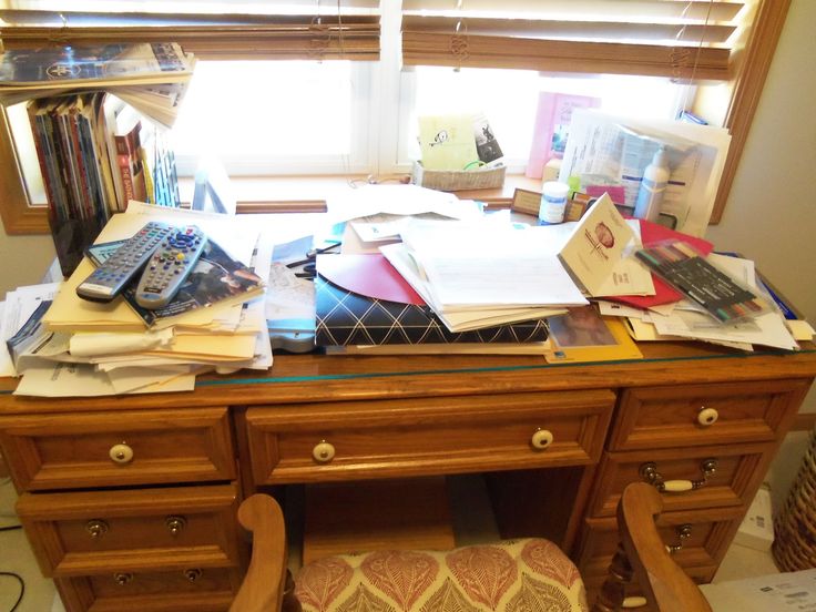
Here is an example. If you have a really small desk, you get to keep it in a small room. But you may have to stack items on top of each other, e.g. books and folders. Pens and pencils may be crammed together in a narrow pen holder. To retrieve one book from the stack, you may need to remove other books on top of it before you reach your desired book. To take out a pen from the holder, you may need to wiggle it out of its crammed space so that it comes unstuck.
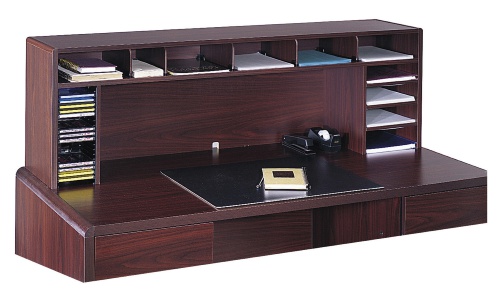
If your desk is large, you’ll need a bigger room. But the items on the desk can be spread out, arranged and sorted. Higher priority items can be put in their own dedicated places so that they are not impeded by low priority items. There can be multiple holders for pens, pencils and other stationary.
Let’s look at the most common types of space complexity algorithms found in the world, both physical and computing
Constant space algorithm
A constant space algorithm is a type of algorithm where space is saved aggressively by restricting the total space taken by the algorithm to fixed number regardless of the number of inputs. The space saving is usually done by restricting the number of inputs used by the algorithm while it runs. The rest of the inputs usually have to wait outside the algorithm in a seperate storage since the algorithm will not entertain them.
A constant space algorithm is a desperate move for devices in which conserving space is the highest priority. A constant space algorithm may be fast per run, since it needs to deal with really less data. But if there is a large number of inputs needing to be processed, a constant space algorithm will have to run several times in a sequence. This leads to a lot of data waiting in queue and slow overall processing time.
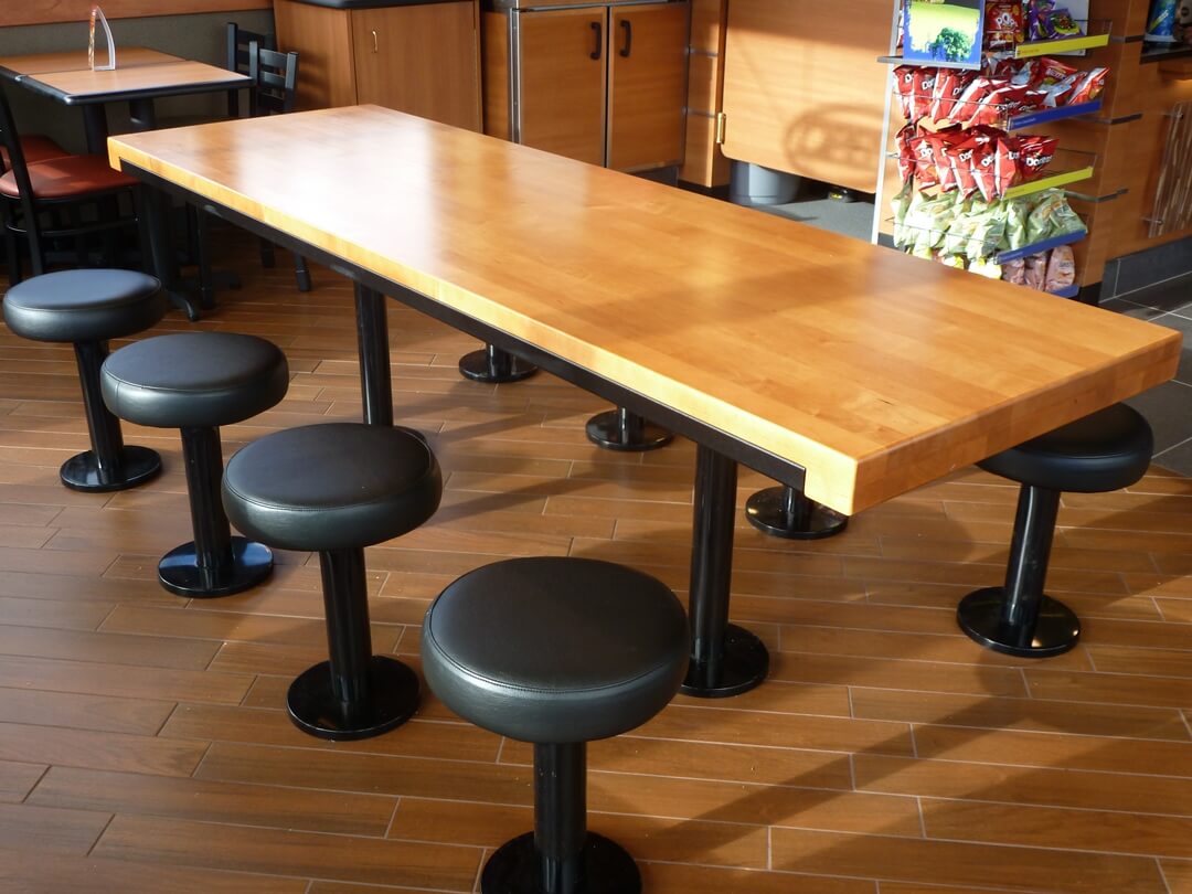
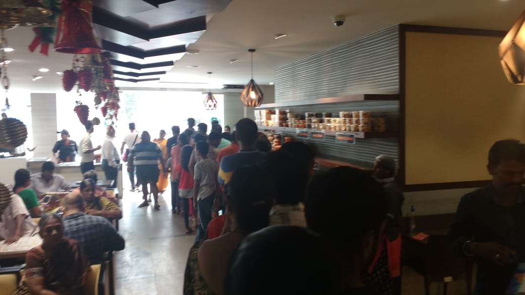
A restaurant is the best way to visualise a constant space algorithm. The restaurant is designed to use the space available to it in the best way possible. So there will be a limited number of tables. They cannot conjure up more tables as footfall increases. As a result, patrons who cannot be accommodated may be turned away or asked to wait. It is possible that the restaurant serves each table really fast. But because of the limited number of tables, patrons may have to wait for a long time to get into the restaurant. Despite their meal being served fast, their overall time spent in the experience might be very high.
Linear space algorithm
A linear space algorithm is the most common algorithm used. It accounts for more than 90% of the algorithms. In a linear space algorithm, the space consumed increases in direct proportion to the number of inputs.
The increase in space consumption may not always be in 1:1 ratio. E.g. it takes 5 envelopes to post 5 letters, since each letter needs an envelope of its own. But it doesn’t take 50 boxes to store 50 visiting cards. Upto 25 visiting cards can sit in one box before the box overflows, requiring you to buy a new box. So the ratio is 25:1. Note that the equation and growth is still linear. It is just that the factor of growth is 1/25, i.e. one unit of storage needs to be consumed for every 25 units of data you have. You’d need 10 boxes to store 250 cards and 20 boxes to store 500. The scale grows in a straight line.
Note that as the ratio grows further apart, it may lead to increasing space wastage. E.g. if you have 27 cards, you’ll still need two boxes, one of them containing 25 and the other holding just 2. An entire box for just 2 cards. 23 spaces lying idle and waste. In such cases, the algorithm can be changed to partition the data to reduce wastage. E.g. what if you used boxes with a capacity of 10 rather than 25? In this case, you’ll need 3 boxes to store 27 cards, but the last box will have 7 cards, leaving a wastage of only 3 spaces.
It is often possible to sample your input data to find storage opportunities with less wastage.
Algorithms growing at more than a linear scale
As mentioned in the paragraph of space-time trade-off, it is possible to arrange data in different shapes and ways to find the best way to work faster with them. E.g. arranging data hierarchically in the shape of a tree, partioning data in variable-sized boxes, arranging data in circular chain, etc.
In these cases, the growth of memory consumption may be more than linear, e.g. quadratic. It totally depends on the data structure used to speed things up.
Let’s take a phone book for instance. A phone book usually has pages with designated letters of the alphabet for each pair of pages. Let’s imagine a small pocket phone book that has 52 pages, each letter given two pages. On each page, there are 10 lines, with each line capable of storing a name and a phone number. So there are 20 names possible for each letter. Letters like ‘A’, ‘S’, ‘T’, ‘M’ and ‘N’ will run out of space very soon. You will find more than 20 contacts for those letters.
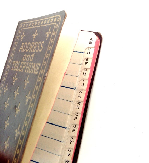
If you have run out of space for just one letter, say for names with ‘A’, you will make some adjustments. E.g. you will use the plenty of space left for letters such as Q or Z. In this case, you are just repurposing and reusing existing space. But if you run out of space for several letters, e.g. ‘A’, ‘S’ and ‘T’, it is unlikely that you will stick all those names into the page with letter ‘Q’, because it damages the meticulous searchability of your phone book. You may consider buying a new bigger phone book with each letter given four pages. In this case, the increase of input caused you to double the storage required.
You may even adjust for a while by sticking a few new blank pages to the end of your phone book and labelling them with the overflowing letters. This will have been a modest increase in the storage, but one that causes you to flip to two sections to look up names for the same letter. The growth of such algorithms depends on the flexibility of the data structure used.
Conclusion
Understanding how an algorithm consumes space and the effects it has on the algorithm’s speed is very important. So is the growth in space consumption that an algorithm requires when input data grows. This is especially important in the world today that works with IoT and small devices with low memory.