A software application is a combination of algorithms working together to do tasks for you. But how can we determine which algorithm to use for a specific problem? One way to choose is by evaluating the time that an algorithm will take to solve a problem and how much memory it will consume. To objectively measure the two quantities, we have two methods called time complexity and space complexity respectively. In this post, we will look at time complexity to determine if our algorithm is fast or slow.

What is an algorithm?

Just like a recipe tells you how to turn raw ingredients into a desired dish using cooking tools /  utensils, an algorithm takes a bunch of data and at least one request that the user wants to fulfill with that data. An algorithm is a sequence of steps that uses the data to answer the user’s request. E.g. when you type the first few digits of a phone number in your phone’s address book, your phone starts narrowing down and showing only those phone numbers that contain the sequence you have typed. This is a search algorithm at work.

While the phone performed a search and returned results, there are several ways to search matching phone numbers from a full list of phone numbers. In the real world and in computers, there is never one right way to solve a problem. There are many ways to do so, but each has benefits and trade-offs. In computing, the main benefits and trade-offs are calculated with regard to the speed of an algorithm, which is the time it takes to complete its work and the amount of memory an algorithm it consumes to work.

Except for rare cases, these two requirements conflict with each other. Usually an algorithm requiring less memory takes more time to run, whereas speedier algorithms consume more memory. Depending on the type of machine you have, you’ll need to select the best suited algorithm among many. This may be the fastest among the algorithms that can fit within a device’s extremely low memory. Or it can be one that consumes the least memory among the algorithms that satisfy your app’s minimum speed requirement.

Measuring methodology

In the world of computing, the speed of a processor is measured in MIPS or million instructions per second. This is an absolute measurement that tells you how many millions of instructions your processor executes every second. This will vary from one machine to another, depending on the capability of the processor.

But not even two computers with identical processors ever execute an algorithm at exactly the same MIPS speed. This is because the two computers may be running other apps that require various levels of attention from the processor. One computer will run the same algorithm at different MIPS speeds depending on what else is running at each moment. A really fast computer may be able to run a woefully inefficient algorithm at a higher MIPS speed than that of a really slow computer running the world’s most efficient algorithm.

As a result, we never measure algorithm speeds in MIPS or even in the time taken in seconds or nanoseconds. Rather, we measure an outcome called ‘complexity’.

Best case, normal case, worst case

Let’s say that we have a deck of playing cards, including the two jokers, making it 54 cards in total. Our request is to find the ace of hearts from the deck. Let’s assume that our algorithm is to pick up each card in the deck, starting from the top, and see if that card is the ace of hearts. If not, then move to the next card in the deck.

The best case of an algorithm is the fastest result. In our case, it would be if the first card we picked up were the ace of hearts. The worst case is if we had to go all the way to the 54th card to find our desired card. Normal case is an average case, i.e. finding the card anywhere between the 20th and the 30th positions.

Complexity

What if we added the diamond-faced cards from a second suite to our original suite? There are 13 diamond cards, thus taking our original deck’s total to 67 (54 + 13). Now suddenly our worst case scenario is 67, i.e, our ace of hearts is found in the last position of our oversized deck.

But what if the cards in the deck are sorted by the number on their faces? All the aces come first, then the twos, then the threes and so on. How does that change our worst cases?

In a deck of 54 cards, there are only 4 aces. In a deck sorted as mentioned, all of them are guaranteed to be within the first 4 positions. So the worst case for finding the ace of hearts is 4. Even if we add the 13 new diamond cards, only one of the new cards will be an ace, i.e. the ace of diamonds. Among the 67 cards, there will be only 5 aces, all guaranteed to be in the first 5 positions. Our worst case will have increased by a single count to 5.

This is exactly what the time complexity of an algorithm measures. Given a bunch of data with ‘n’ items, what is the worst case when you run a particular algorithm? And if we increase the number of items in a set, does the worst case increase too and by how much does it increase? Why is it called time complexity when it relates to the number of items? That’s because the worst case mentions the number of items that have to be processed before arriving at a result. We can easily infer that an algorithm that processes more items takes more time. E.g. finding the ace of hearts at the 54th attempt clearly takes way more time that finding it at the 4th.

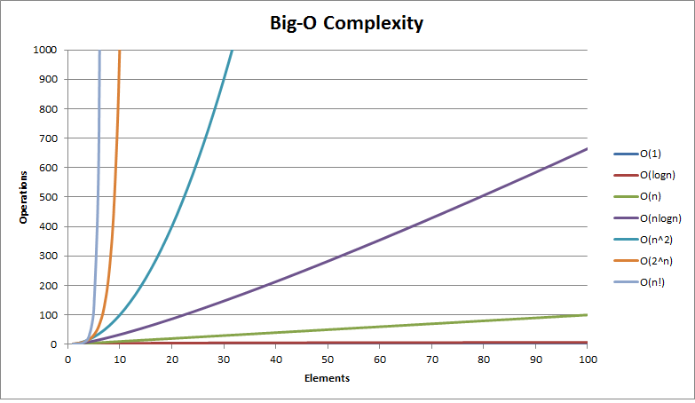
O-notation

Without being too detailed, let me introduce to you that time complexity is represented using a indicator called the O-notation. The capital O is followed by a bracket that either has the number 1 or the symbol n with some mathematical variation. Here is how you read an O-notation indicator.

O(n) = The algorithm scales to the order of n.
O(n³) = The algorithm scales to the order of n³.

Without confusing you with mathematics, here are most common algorithm complexities with day-to-day examples.

O(1)

O(1) is the most efficient complexity for an algorithm. It says that the worst case time is not affected by adding more items to our data set. There are no wasted efforts or trial and error. Here is a real life example.

Let’s say that you are using a phone book with tabs that indicate pages dedicated to specific alphabets. Since the alphabet is visible, there is no trial and error. You slide a finger under a tab and directly flip to the alphabet page you want. It doesn’t matter if you want to jump to letter ‘A’ or ‘Q’. There is exactly one step for each. English has 26 alphabets. What if we use a language like Hindi which as more than 40 different characters? It wouldn’t matter as long as each character has a tab that you can slide your finger over and flip directly to the desired page.

O(1) algorithms are a programmer’s dream, but they usually take up plenty of memory. We’ll see why in a post about space complexity.

O(log n)

What if you want to look up the word ‘equity’ from an Oxford dictionary. The dictionary is guaranteed to be sorted alphabetically, so you can rest assured that ‘a’ will come before ‘z’, ‘summer’ will come before ‘winter’ and interestingly ‘Wednesday’ will come before ‘Tuesday’.

How do you typically use a dictionary? We know that the letter ‘e’ has to be in the first half of the dictionary, since as the 5th alphabet, it appears closer to the start. You slide a finger somewhere in the middle of the starting half of the dictionary and arrive on the page that says ‘hedge’. Well, since ‘e’ appears before ‘h’, you need to go left. In the process, you completely eliminate everything to the right of ‘hedge’. By how our data set is designed, our target can only be in one direction and not the other.

After a couple of more finger sliding attempts and elimination, you will arrive at ‘equity’. Note that at every step, you are eliminating one side of your dataset and zeroing in on the other side. Such as algorithm is called O(log n) algorithm. Because as the worst case, it takes as many steps to nail your search as the value of n’s logarithm to the base 2. Note that since we are in the binary world, our base will be 2 and not ‘e’ as used in physics. E.g. Finding a target in a set of data that has 32 items will at most take 5 steps.

O(n)

In O(n), the complexity is exactly the same as the size of data. Our example about the unsorted deck of cards in the paragraph about complexity is an example of O(n). The worst case for 54 cards was 54 and that for 67 cards was 67.

Just for completeness, the complexity for the sorted deck of cards is somewhere between O(1) and O(log n), i.e. neither ideally efficient as O(1), but far better than O(log n).

O (n log n)

While search algorithms do not take higher complexities like n log n, other algorithms, such as that for sorting a deck of cards in some order, come under the n log n category. To sort a deck completely, you need to go over the deck multiple times until the sorting is done.

O(n²)

Problems where we need to pair items from two sets often lead to n-squared complexity. E.g. matching 5 keys to 5 door key holes is an n-squared complex problem.

O(2ⁿ), O(n!)

There are called exponential and factorial complexities. Ideally you should never write algorithms that perform at these complexities since they seem to take eternity. If your measurement shows these complexities, then you have written something inefficient and the code must be refactored.

Conclusion

Time complexity is a useful study since you want your app to perform at its best and not slow down because an algorithm you have chosen is inefficient. The more you practise it, the more you get better at evaluating algorithms quickly.